Introduction to High-Performance Computing (HPC)#
High-Performance Computing (HPC) refers to the use of supercomputers or parallel computing techniques to perform complex computations quickly. HPC systems aggregate computing resources to solve problems that would be unfeasible or time-consuming using conventional methods. These systems play a critical role in research fields like bioinformatics, physics, climate modeling, and engineering.
Why Use HPC?#
High-Performance computing is a game-changer for tackling some of the most challenging problems today in science, engineering, and data analysis. Imagine you are working with a data set so large that a normal desktop computer would take days to weeks to process it - HPCs are able to handle the task in hours or even minutes because of the combined power of many interconnected processors and computers, enabling the simultaneous processing of data. For example, fields like genomics rely on HPC to analyse DNA sequences across entire populations, while climate scientists use it to model weather patterns with high accuracy. Similarly, researchers working on optimisation problems, such as desgigning efficient supply chains or fluid dynamics depend on HPC to handle the scale of calculations involved in their modelling.
But how do HPCs achieve better results in less time? This is because of parallel computing, which is the ability to divide large tasks into smaller pieces that can be completed simultaneously. You can think of this like a group of people working together to build a house - each person has a specific task which they work on at the same time, finishing the job faster. In genomics, for example, modern sequence alignment methods align genomes by splitting up the sequences, and aligning individual chunks to each other until they are successfully aligned, in parallel - a much more efficient method than loading entire genomes (hundreds of millions, to even billions of nucleotides) and placing each genome alongside another to match it, sequentially.
So, when should you consider using HPC?
If you’re running simulations that require thousands of iterations—like predicting how a hurricane might behave over time—or working with massive datasets, such as analyzing millions of genomic sequences, HPC is essential.
It’s also a great choice when your tasks can be automated, like running multiple models or simulations at once, freeing you to focus on interpreting the results. HPC systems are particularly powerful for long-running tasks that demand significant memory or computational power, making them ideal for tasks that go far beyond the capabilities of standard desktop computers.
By mastering key high-performance computing concepts, you’ll gain an understanding of how problems can be approached more efficiently, tackle larger datasets, and expand the scale of what’s possible in your field.
Key Computer Hardware Vocabulary#
It’s good to first familiarise yourself with some computer hardware terms that are frequently used. Whether you’re running code locally or on an HPC, you can run into limitations with system you are using, informing not only your methods development and hardware optimisation, but also allows you to troubleshoot performance issues and make informed decisions about how to structure your computational tasks.
CPU (Central Processing Unit) – Often referred to as the computer’s “brain,” the CPU is responsible for executing instructions, managing data, and interacting with memory. In all modern computers, including HPCs, CPUs consist of multiple cores that allow for the simultaneous execution of multiple instructions.
CPU Core – A core is a processing unit within a CPU that can execute instructions independently. Cores are designed to handle multiple threads, enabling more efficient processing of tasks. Each core and thread can execute its own set of instructions, allowing for parallel execution of workloads, which is essential for complex computations and multitasking.
Thread – A thread is the smallest unit of execution within a process. In most modern high-performance computing (HPC) systems, processes are divided into threads rather than cores, allowing for efficient resource utilisation through multithreading. This enables multiple threads to run concurrently, maximising CPU utilisation and speeding up tasks like data processing, simulations, and scientific computations.
GPU (Graphics Processing Unit) – Initially developed to manage visual tasks, GPUs are now widely used in parallel programming for handling large volumes of basic arithmetic operations, primarily through matrix multiplications. They are highly efficient at processing many calculations simultaneously, making them ideal for scientific computations and machine learning applications.
Random Access Memory (RAM) – Usually referred to as just “memory”, RAM is the temporary storage that the CPU uses to hold data actively being processed. RAM allows for quick access to data needed for computations, which is either deleted or deposited into NVM storage once completed.
Non-Volatile Memory (NVM) - Non-volatile memory refers to any form of memory that retains data even when the system is powered off. This includes storage devices like hard drives (HDDs), solid-state drives (SSDs), and flash drives. Unlike RAM, which is cleared when the system shuts down, NVM provides long-term data storage, allowing for the preservation of files, applications, and system states across power cycles.
HPC Systems#
Clusters#
An HPC cluster is a collection of interconnected computers (nodes) that work together. Each node in a cluster is typically a standard server or workstation, but together they behave as a single powerful system. Clusters are commonly used in scientific research because they can be built using off-the-shelf hardware.
Supercomputers#
Supercomputers are specialised machines designed for high-speed computations. They consist of thousands (or even millions) of processors working together to complete a single task, often composed of many cluster nodes or purpose-built platforms (e.g., NVIDIA DGX GH200) . They are optimised for performance, providing the highest level of computational power.
Distributed Systems#
Distributed systems consist of computers that are geographically spread but connected over a network. These systems allow for distributed computing, where different parts of a computation are handled by different machines. Drawbacks of this include data transfer, a
Serial vs Parallel Processing#
Serial Processing#
Serial (or sequential) programming is the execution of tasks in a step-by-step, linear sequence where only one instruction is processed at a time. In this model, the processor completes one task before starting the next, with no overlap or concurrency. While this method is simple and efficient for small, straightforward tasks, it becomes a bottleneck for larger problems requiring extensive computation.
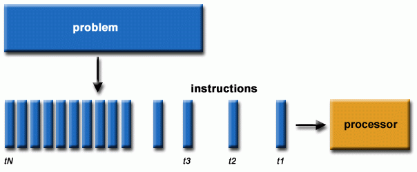
Fig. 34 Serial programming chain of operations (https://hpc.llnl.gov/training/tutorials/introduction-parallel-computing-tutorial)#
Parallel Processing#
At the heart of HPC is parallel computing, where multiple calculations or processes are performed simultaneously. This is typically achieved by dividing tasks among multiple processors, which work together to complete a job faster than a single processor could.
A frequent misunderstanding is that executing code on a cluster will automatically result in improved performance. Clusters do not inherently accelerate code execution; for enhanced performance, the code must be explicitly adapted for parallel processing, a task that falls under your responsibility as a programmer.
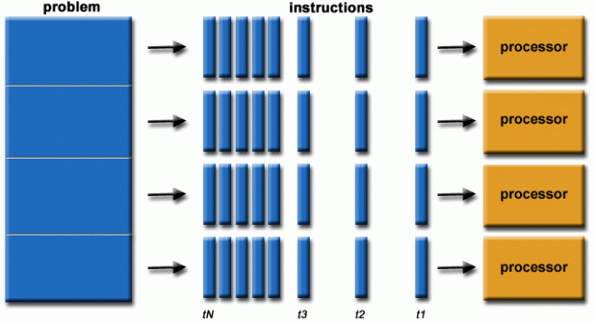
Fig. 35 Parallel programming chain of operations (https://hpc.llnl.gov/training/tutorials/introduction-parallel-computing-tutorial)#
Types of Parallelism#
Data Parallelism: Divides large datasets into smaller chunks, which are processed simultaneously. Each processor works on a different piece of data.
Task Parallelism: Different processors perform different tasks simultaneously. Each processor works on a separate part of the overall computation.
Hybrid Parallelism: A combination of both data and task parallelism, where both the tasks and data are split across multiple processors.
HPC Workflows and Use Cases#
Embarrassingly Parallel Tasks#
Some tasks are naturally suited for parallelisation, often referred to as “embarrassingly parallel.” This means that each part of the task can be executed independently without any need for communication between processors. Examples include:
Image rendering: Each pixel or frame can be calculated separately.
Monte Carlo simulations: Each iteration is independent of the others.
High Throughput Computing (HTC)#
In some cases, a large number of relatively simple operations need to be performed. High-throughput computing is a paradigm where many independent jobs are processed concurrently. This is useful in:
Bioinformatics: Performing sequence alignments or genome annotations.
Data processing: Handling large datasets where each piece can be processed individually.
Memory-Intensive Tasks#
HPC systems are ideal for tasks that require more memory than is available on a local machine. Large-scale data analysis or the visualisation of vast datasets often requires enormous amounts of memory.
Job Arrays#
A job array consists of multiple “tasks” that perform the same job but with different parameters or datasets. This approach is especially useful when you have many independent simulations, analyses, or calculations that can run in parallel.
Job arrays are an essential feature of HPC systems that allow users to submit a large number of similar tasks simultaneously. Instead of submitting multiple jobs manually, you can use a job array to submit a series of jobs with a single command.
For example, imagine you need to run the same simulation 100 times with different input parameters. Instead of submitting 100 individual jobs, you can create a job array that runs all the simulations simultaneously.
Trade-offs#
While HPC provides tremendous computational power, there are some trade-offs:
Setup Time: Configuring jobs on an HPC cluster can be time-consuming, requiring careful management of resources such as memory, CPU, and runtime limits.
Parallelisation Overhead: Not all tasks benefit equally from parallelisation. In some cases, the overhead involved in coordinating multiple processors may diminish the performance gains.
Learning Curve: Using HPC often requires learning job submission systems (e.g., Slurm, PBS) and optimising code for parallel execution, which may be challenging for new users.
It is important to consider the extent of realised gains of parallelisation when using HPC systems. The ideal setup of any computing system would allow for scalable parallelisation in which doubling the number of processes will double the speed of a job. Amdahl’s Law allows us to predict theoretical speedups in parallelised computing jobs, where the idealised speedup scales almost linearly with increasing division of labor across processors, but is ultimately restricted by the portion of the program that cannot be parallelised.
In real life, gains under Amdahl’s Law cannot be realised. As programmers looking to parallelise our work, we have to take into consideration computer structures, and primarily their latency in transferring data across systems. All networks, whether they are between cores, processors, nodes, or entire clusters, have non-zero transfer latency and limited bandwidth, meaning the speed of communication between them does not happen infinitely fast.
We can expect that the more we split processes, the more that latency issues will reduce the efficiency of parallelisation, especially as the complexity of the system increases.
Shown in the example figure below, we see minimal trade-offs from ideal speedups from 1-16 cores in this system they increase as we escape from the smaller bounds of core-core latency and reach cpu-cpu latency at 32, with significant bottlenecks after 128 threads where we use 7 whole compute nodes (i.e. 7 separate computers)!
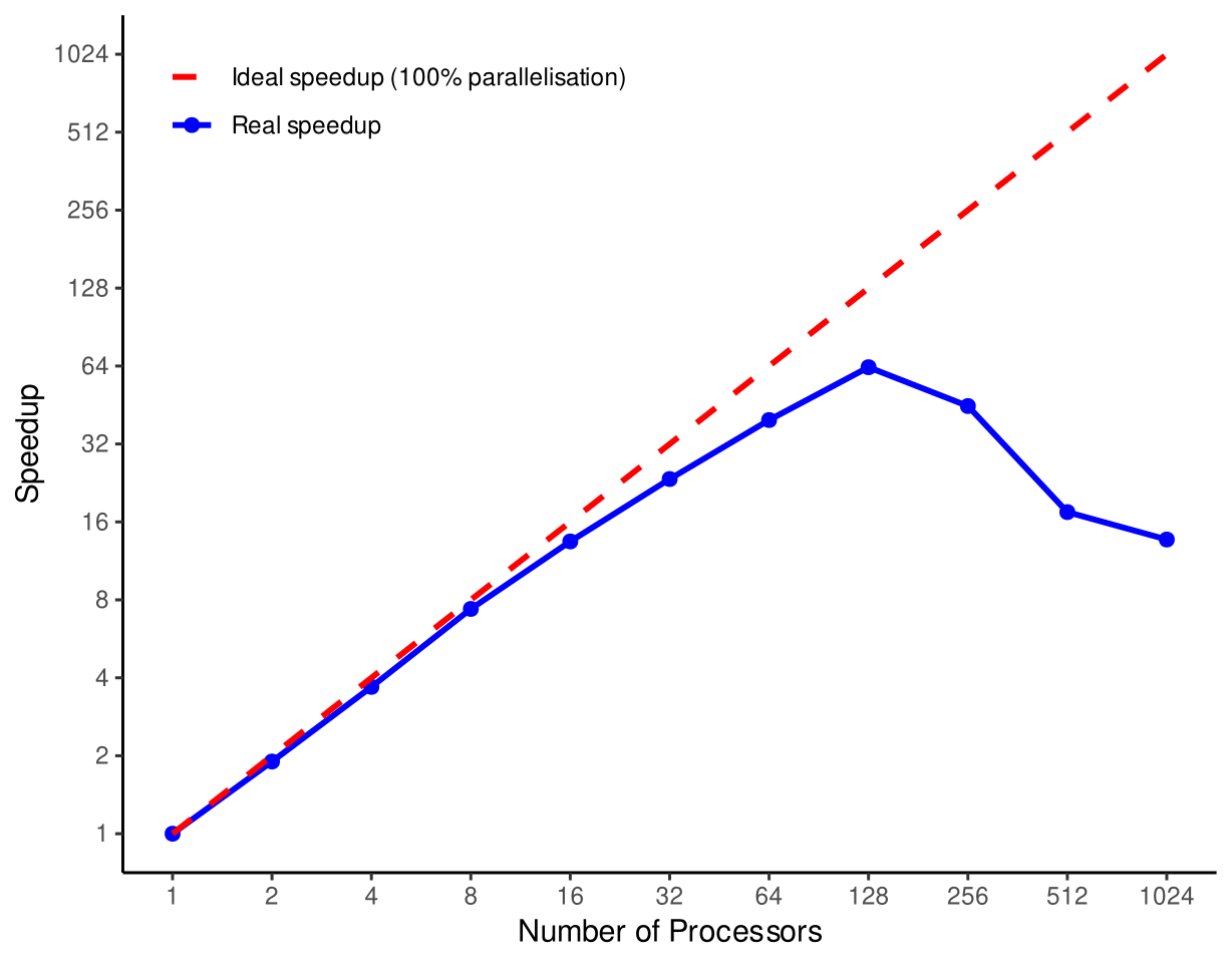
Fig. 36 Speedup achieved from ideal parallelisation vs realised (Data from: https://hpc-wiki.info/hpc/Scaling)#
The realised speedup diverges so much from ideal because of the increased latency in communicating and transferring data between the many nodes used in this system.
This divergence can occur on smaller scales, not just between nodes, where we may have a CPU with hundreds of threads - just take a look at one of the latest processor’s from AMD, for example the EPYC 9965, each having over 384 threads. The distribution of information across that many independent pathways can be a struggle, and should be considered when designing parallelisation workflows.
Local Parallelisation#
Local parallelisation on a laptop, desktop, or workstation can significantly improve performance by harnessing the full potential of multi-core CPUs in a controlled environment. While HPCs are tailored for massive computations, local parallelisation on personal devices offers the ability to speed up individual, day-to-day applications.
Parallelising your code locally is ideal for repetitive computations or simulations, such as running the same model on different datasets, bootstrapping analyses, or performing parameter sweeps. By dividing each repetition across cores, you can perform these tasks simultaneously rather than sequentially, reducing execution time significantly. This is particularly useful for tasks like cross-validation or Monte Carlo simulations, where each iteration is independent and benefits from being run in parallel.
In R, the
parallelpackage gives us access to parallelisation functions, such asmclapply(multi-corelapply) Additional packages include future and foreach.Python also has powerful libraries for parallel computing, such as
multiprocessingandconcurrent.futures. Both libraries provide straightforward ways to parallelise tasks locally.
Below is an example of parallelised model fitting using mclapply in
the parallel package in R. In this code chunk, we generate example
data that is grouped by an ID column and we want to apply a linear
model to each ID group. First we can generate the data:
n <- 10000   # Number of observations

data <- data.frame(
  ID = sample(1:10, n, replace = TRUE),  # ID column to define 10 groups
  y = rnorm(n),
  X = rnorm(n)
)
We can then split the data into a list of data sets, which allows us to
use a list-apply function like lapply/mclapply, and define our
function for outputting the coefficients for the corresponding ID
group:
library(dplyr)

data_groups <- data %>% group_by(ID) %>% group_split() # Split the data by ID

# Define a function to fit a linear model for each group
fit_model <- function(group_data) {
  model <- lm(y ~ X, data = group_data)
  coef_df <- as.data.frame(t(coef(model)))
  coef_df$ID <- unique(group_data$ID)  # Add ID for reference
  return(coef_df)
}
Finally, we should parallelise the code by identifying the number of
cores our system has, avoiding hard coding this information - keep this
in mind if you want others to run it on a different system! We may also
want to leave one core for general system processes. As we have applied
this onto a list we want to consider bringing this information back
together, using a function like bind_rows.
library(parallel)

num_cores <- detectCores() - 1 # Use all cores but one

results <- mclapply(data_groups, fit_model, mc.cores = num_cores) # Fit the models

final_results <- bind_rows(results) # Bind model outputs from list to table
print(final_results)
Getting Set Up on the Imperial HPC#
You can find all information about getting started and working on the Imperial HPC here: icl-rcs-user-guide.readthedocs.io
To get started, you will need 4 things:
Access to the HPC system: You should have received an email from noreply@imperial.ac.uk with the subject heading “Welcome from the Research Computing Service”. If you have not received this email, please let me know as soon as possible so we can try and get you added this week.
A method of working on the cluster: The cluster is accessed using Secure Shell (SSH). If you are using Linux or macOS then you should have OpenSSH already installed alongside your operating system, which can be accessed from a terminal session such as command prompt. You can double check that this is available to you by logging into the HPC service for the first time. In a terminal session, enter the following, substituting your own username (in the form abc123), and entering your Imperial password when prompted:
sftp username@login.hpc.imperial.ac.uk
If this has been successful, you will see a message containing the title “Imperial College London Research Computing Service”
Necessary modules are set up in your remote are: It will be useful to ensure that Python and R are set up on your area of the HPC system at this stage. You will only need to do this once. To install Python and R, you will need to first log in to the HPC service (as covered in the above section), and then enter the following two lines into the command line within your area of the remote system:
module load anaconda3/personal
anaconda-setup
This could take some time and may require you to respond “yes” when prompted. Once anaconda is fully installed, install R by entering
conda install R
Once again, this could take some time and may require you to respond “yes” when prompted. Once both of these are installed, you should be able to enter python3 and code in Python on the cluster node. However, in general you should only run code in either R or Python by submitting them within jobs (as covered in the lectures and in the instructions document). (You will notice that if you attempt to launch R from your HPC node you will be given a stern message!)
A method of file transfer: Files are exchanged between your local machine and your area on the HPC system using Secure File Transfer Protocol (SFTP). If you are working in Linux or macOS, you should be able to achieve this directly from the terminal. To check this, enter the following and enter your password when prompted:
sftp username@login.hpc.imperial.ac.ukOnce you are logged in, type and enter pwd to find out which area of the system you are in. By default you should land in username$HOME, and by entering put filename.R this file should be copied from your current local directory to your current remote directory. You can also similarly use the Secure Copy (SCP) method to transfer files – this, and further information about copying and getting files to/from the remote directory, will be covered in the main instruction document
Running a job on the Imperial HPC#
You first must determine the task at hand. Are you running your own script or software that natively parallelises tasks? Is your job an array?
Using arrays as an example, we would first want to make an R or Python
script that takes in a job number and uses that to determine which task
to perform. The HPC_script.R/py files below, when sourced, identify
the job number (that is, the job number the Imperial HPC assigns to our
code submission), run our code, and then save the outputs to the current
working directory, with all file names being distinct (otherwise the
different jobs will overwrite each other).
In R:
seed_number <- as.numeric(Sys.getenv("PBS_ARRAY_INDEX")) # Find out the job number

set.seed(seed_number) # Set this as the random seed so that all runs have a unique seed

output <- runif(n=10000,min=0,max=1) # # Run whatever simulation we want

save(output,file=paste("output_",seed_number,".rda")) # Save this to a file

rm(output,seed_number) # Remove our objects from the environment
Similarly, in Python:
seed_number = int(os.getenv("PBS_ARRAY_INDEX")) # Find out the job number

seed(seed_number) # Set this as the random seed so that all runs have a unique seed

output = numpy.random.uniform(0,1,1000) # Run whatever simulation we want

with open(print("output_",str(seed_number),".data",sep=""),"w") as f:
  f.write(output) # Save this to a file

del seed_number # Remove our objects from the environment
del output
Using SFTP or SCP from the terminal of your local machine, copy your
task script to an area on the remote machine (e.g.,
$HOME/HPC_script.R).
To run your job on the HPC, you must write a .sh file to provide the cluster with instructions to run the task script. This will reference your task script, so you will need to be mindful of the relative file path. This file must contain the following fields at the top:
#!/bin/bash
#PBS -l select=N:ncpus=X:mem=Ygb
#PBS -l walltime=HH:00:00
This will determine the queue that your job gets put into. If your requested specifications do not fall within at least one queue, your job won’t run! Have a look at the RCS job sizing guidance for more information.
Within this file, you will generally want to load any modules and
packages, print any statements to check your progress within the job
output files, and transfer files to and from the job to your working
directory. For your outputs to be created correctly, you must move
your files to $TMPDIR to be processed, and then move files from this
back to $HOME. This is because $TMPDIR is where your files are
run, whereas $HOME is where you interact with them!
This can be summarised in the run_script.sh file below, where we are
running the HPC_script.R file from above. Because the R script does
not parallelise within it and does not load a significant amount of
data, we will only request a single thread (ncpus) and 1GB of RAM
(mem):
#!/bin/bash
#PBS -l walltime=12:00:00
#PBS -l select=1:ncpus=1:mem=1gb

module load anaconda3/personal

echo "R is about to run"

cp $HOME/HPC_script.R $TMPDIR

R --vanilla < $TMPDIR/HPC_script.R

mv $TMPDIR/output_* $HOME/output_files/

echo "R has finished running"
The Imperial HPC uses the PBS Pro job scheduler (documentation available
here),
whereas other systems may use SLURM (documentation available
here). To submit your
job to the queue you will use the qsub command. If you are submitting
an array job, as we are with run_script.sh, you want to use the -J
option and specify the number of jobs to run. In this case:
qsub -J 1-32 run_script.sh (tells the cluster to do 32 runs based on
the .sh file - the job number will be from 1-32). Additionally:
qstat- tells you the job ID and its current statusqdel jobID- cancels the jobcat filename.sh.ejobID- are error files empty?cat filename.sh.ojobID- are standard output files as expected?