Introduction to Jupyter

Introduction to Jupyter#

What is Jupyter?#

The Jupyter Notebook offers an interactive interface to multiple programming languages (including Python and R) that can be viewed and manipulated in web browsers.

Jupyter notebooks can run code, and also store the code and a current snapshot of the output (graphics and text), together with notes (in markdown), in an editable document called a notebook (like this one you are currently reading).

Thus a Jupyter notebook is similar to a Mathematica or Maple notebook. The difference is that Jupyter is free, fast improving, and unlike Mathematica or Maple notebooks, the Jupyter notebook can support over 100 programming languages (more on this below). Furthermore, Jupyter notebooks are saved on disk as a JSON files (with a .ipynb extension), so are fully open source and can be kept under version control.

Why use interactive notebooks?#

Jupyter is a great tool for “literate programming”; a software development style pioneered by (yes, again!) Donald Knuth. In his words:

Let us change our traditional attitude to the construction of programs: Instead of imagining that our main task is to instruct a computer what to do, let us concentrate rather on explaining to human beings what we want a computer to do.

In literate programming, human-friendly text is as important as code, making coding accessible to a larger proportion of people.

And just as importantly, literate programming also helps address the generally poor reproducibility of scientific research by making your code and your methods better reproducible and reusable.

With Jupyter notebooks, you can explore quantitative ideas by combining snippets of computer code and human text. The main uses of Jupyter notebooks are:

Data science (e.g., with pandas)
Mathematical analyses (e.g., with sympy)
Interactive visualization (e.g., with matplotlib or ggplot)
Education and teaching
Research communication and reproducibility

Jupyter Notebooks are increasingly being used as a research and teaching tool in academic institutions, government agencies (e.g., NASA, LIGO), as well as industry sectors (e.g., Google, Netflix, Bloomberg).

Key Jupyter features#

The Jupyter Notebook:

…allows you to keep notes using markdown, the increasingly popular markup language.
…offers features available in typical Interactive Development Environments (IDEs) such as code completion and easy access to help.
…has LaTeX support.
…can be saved and easily shared in the .ipynb JSON (JavaScript Object Notation – syntax for storing and exchanging data).
…can be kept under version control (e.g., with git).
…can be rendered and viewed online (e.g., on GitHub).
…can be exported to multiple formats, including html, pdf, and slides.

Jupyter vs. IPython#

Brian Granger and Fernando Pérez created IPython (Interactive Python) as an implementation of Python for literate programming, taking advantage of improved web browser technologies (e.g., HTML5). IPython notebooks quickly gained popularity (they were a great alternative to Mathematica and Maple as well), and in 2013 the IPython team won a Sloan Foundation Grant to accelerate development of this technology. The IPython Notebook concept was expanded upon to allow for additional programming languages, which became project Jupyter (why “Jupyter”? See this). IPython itself is now focused on the interactive Python project per se, part of which is providing a Python kernel for Jupyter.

Your Jupyter notebooks will typically open in IPython as well, but will not allow you Jupyter-only features (of course!)

Installing Jupyter#

Please see project Jupyter’s instructions for installation. Also, see this.

Modern Jupyter Interfaces#

While this tutorial focuses on Jupyter Notebook, you should be aware of modern alternatives:

JupyterLab: The next-generation interface for Jupyter, now the recommended default. It provides a more flexible, IDE-like environment with tabs, file browser, and extensible interface. Install with: pip install jupyterlab and launch with: jupyter lab
VS Code Jupyter Extension: VS Code provides excellent built-in support for Jupyter notebooks with features like IntelliSense, debugging, Git integration, and no need for a separate browser. This is covered in detail below.
Classic Jupyter Notebook: The original interface (covered in this tutorial), still widely used and great for learning the basics.

Installing and running jupyter in a virtual environment#

It is recommended that you install Jupyter in a virtual environment (like venv) on Ubuntu or macOS because:

Dependency Isolation: Jupyter requires various Python packages (like notebook, ipykernel, and others), which may depend on specific versions of libraries. By installing Jupyter in a virtual environment, you avoid conflicts between versions of these libraries that other projects or system applications might require. This isolation ensures that your Jupyter environment runs smoothly without interfering with or being affected by other Python projects.
Easy Upgrades and Uninstallations: Virtual environments allow you to manage, upgrade, or uninstall packages without affecting the global Python environment. You can test updates to Jupyter or other libraries without risk to your system’s stability.
Security: Running Jupyter in a virtual environment minimizes security risks, as it reduces the exposure of the system’s core libraries to potentially vulnerable or outdated packages. If something goes wrong, the impact is contained within the virtual environment.
Environment Customization: Different projects may require specific versions of Jupyter or different sets of dependencies. By using virtual environments, you can easily switch between environments tailored for each project, helping to maintain consistency across teams or over time.

This setup is particularly useful for data science and software development workflows, where dependencies and library versions change frequently.

Ubuntu/Linux Installation#

Here are the steps to use venv to install and run Jupyter on Ubuntu:

Install Python and venv (if not already installed):

sudo apt update
sudo apt install python3-venv -y

Tip

The -y flag in the apt command on Ubuntu (and other Debian-based systems) automatically answers “yes” to any prompts that would normally appear during the installation, upgrade, or removal process. This is particularly useful when scripting installations, as it allows apt to run non-interactively without waiting for user input to confirm actions.

Create a virtual environment:
```
python3 -m venv myenv
```

Note

This will automatically create a myenv directory in your current location. You can create it in your home directory: python3 -m venv ~/myenv. Check this by using ls ~/

Activate the virtual environment:
```
source ~/myenv/bin/activate
```
Install Jupyter within the virtual environment:
```
pip install jupyter
```
Or for JupyterLab (recommended):
```
pip install jupyterlab
```
(Optional) Deactivate the Virtual Environment:

When you’re done installing / running (see below) jupyter, you can deactivate the virtual environment with:
```
deactivate
```

macOS Installation#

The process is very similar on macOS, with a few platform-specific notes:

Install Python (if not already installed):

Python 3 comes pre-installed on recent macOS versions. Check with:
```
python3 --version
```
If you need to install or update Python, use Homebrew:
```
brew install python3
```
Create a virtual environment:
```
python3 -m venv myenv
```
Or in your home directory:
```
python3 -m venv ~/myenv
```
Activate the virtual environment:
```
source ~/myenv/bin/activate
```

Note

On macOS, you’ll see (myenv) prepended to your terminal prompt when the environment is active, just like on Linux.

Install Jupyter:

pip install jupyter

Or for JupyterLab:

pip install jupyterlab

Deactivate when done:
```
deactivate
```

Tip

macOS users: If you’re using the default Terminal app, the activation command works the same as on Linux. If you’re using zsh (the default shell on macOS Catalina and later), the activation process is identical.

Language Kernels#

See this for instructions for installing the Python and R kernels. Or you can go through here (and install additional language kernels if you want).

Adding extensions to Jupyter#

Again, see this for installing jupyter extensions.

Launching/Running a Jupyter Notebook#

In Linux / Mac, Jupyter will start in the directory that you launch it from through terminal. So in your terminal first cd to your weekly coursework’s code directory. Then, simply launch jupyter (Linux / Mac):

jupyter notebook

This will initialize a new server instance (watch your active terminal) and launch a web browser with the Jupyter interface, including a menu at the top.

Play around a bit. For starters,

\(\star\) Create a new nb called MyFirstJupyterNb.ipynb using the menu in your code directory.

Once you have created the new nb, you can launch it next time by cd’ing to its location and then launching it by name:

jupyter notebook MyFirstJupyterNb.ipynb

Note

macOS users: The process is identical on macOS. The terminal commands work the same whether you’re using the default Terminal app, iTerm2, or any other terminal emulator. Just make sure you’ve activated your virtual environment first if you’re using one.

Using `tmux`#

You may notice that jupyter locks up the terminal you launch it from until it is closed. This can be particularly frustrating, and there is an elegant solution. Enter tmux!

tmux is a “terminal multiplexer”, allowing you to run terminal sessions independent of (or “detached” from) a terminal window. You can install tmux using apt:

sudo apt install tmux

Detaching and Reattaching#

To run jupyter in a tmux session, start tmux using the command tmux. From here you can use the tmux terminal as you would your usual terminal session (so launch jupyter notebook as before), however if at any time you decide that you want to do something else, you can detach.

To detach your terminal window from the session, use the shortcut ctrl+b, d (ctrl+b, then let go of that and hit d). This kicks you back to the normal terminal, however your other session is still running in the background.

To see which sessions are currently running, use

tmux ls

And to attach to the session:

tmux a

Note: you can attach to a session from a different terminal window or even terminal program!

To quit tmux entirely, just quit the terminal session either with ctrl+d or exit

Why use `tmux`?#

While this is mostly just a quality of life suggestion, countless are the times that I have accidentally closed my terminal only to find that my jupyter session has also died. By decoupling the window from the terminal session, this no longer happens.

Additionally tmux is absolutely invaluable when running long jobs on a remote server. In this case you can simply disconnect from the tmux session on the remote server. Then you can log in later (and/or from a different computer) and reattach to the interactive session (using tmux a) to check progress. In combination with good logging for long jobs, this can make your life infinitely easier.

Using Jupyter in VS Code#

Visual Studio Code provides excellent built-in support for Jupyter notebooks, offering a modern alternative to the browser-based interface. This approach is increasingly popular in educational and professional settings.

Advantages of VS Code for Jupyter#

Integrated Development Environment: Work with notebooks, scripts, and terminal all in one window
IntelliSense: Advanced code completion and suggestions as you type
Debugging: Full debugging support with breakpoints in notebook cells
Git Integration: Built-in version control without leaving the editor
No Browser Required: Everything runs within VS Code
Variable Explorer: View and inspect variables without printing them
Outline View: Navigate large notebooks easily using the outline sidebar

Setting Up Jupyter in VS Code#

Install VS Code: Download from code.visualstudio.com
Install Python Extension:
- Open VS Code
- Click the Extensions icon (or press Ctrl+Shift+X / Cmd+Shift+X on Mac)
- Search for “Python”
- Install the official Microsoft Python extension (this includes Jupyter support)

Install Jupyter:

pip install jupyter ipykernel

Or if using a virtual environment:

source ~/myenv/bin/activate  # macOS/Linux
pip install jupyter ipykernel

Select Python Interpreter:
- Open VS Code
- Press Ctrl+Shift+P / Cmd+Shift+P (Mac) to open Command Palette
- Type “Python: Select Interpreter”
- Choose your Python installation or virtual environment

Creating and Running Notebooks in VS Code#

Create a New Notebook:
- Press Ctrl+Shift+P / Cmd+Shift+P (Mac)
- Type “Create: New Jupyter Notebook”
- Or create a file with .ipynb extension
Run Cells:
- Click the ▶️ play button next to each cell
- Or press Shift+Enter to run cell and move to next
- Or press Ctrl+Enter / Cmd+Enter (Mac) to run cell and stay
Add Cells:
- Hover between cells and click + Code or + Markdown
- Or use keyboard shortcuts similar to classic Jupyter

VS Code-Specific Features#

Variable Explorer: Click the “Variables” button at the top of the notebook to view all variables
Outline: Use the outline view in the sidebar to navigate to specific cells
Cell Toolbar: Each cell has a toolbar with options for cell type, run, debug, etc.
Notebook Diff: View differences between notebook versions with Git integration
Interactive Window: Run Python scripts interactively with #%% cell markers

Tips for macOS Users#

Use Cmd instead of Ctrl for most shortcuts
Terminal integration works seamlessly with both bash and zsh
VS Code respects your system Python installations and virtual environments
For best performance, add VS Code to your Dock for quick access

Note

VS Code’s Jupyter support is particularly useful when working on coursework that involves both code development and notebook-based analysis, as you can switch between files without changing applications.

Key elements of the Jupyter nb content#

The two main elements (and the associated syntax) you need to know to modify the content of a Jupyter nb are as follows. These will either be entered into text-only cells (“markdown cells”), or code cells. To insert a new cell, click on the edge of an existing cell, and hit A or B on your keyboard to insert a cell above and below, respectively. By default, Jupyter inserts a code cell. To convert it to a text cell, hit M immediately after inserting the cell, or if you have clicked elsewhere after inserting the cell, by clicking on the edge of the new cell and then hitting M. You can now either enter and modify text or code:

Text cells#

Text is formatted using markdown and standard html. The markdown cheatsheet for github is very handy. Give it a quick spin to get started with markdown.

Equations#

You can insert inline or standalone equations by using standard \(\LaTeX\) environments (and you can access more \(\LaTeX\) functionality and environments using the LaTeX_envs extension.). For example, how about the ecologist’s beloved logistic growth equation:

$$
    \frac{dN}{dt} = rN \left( 1-\frac{N}{K}\right)
$$

which will render as:

\[\frac{dN}{dt} = rN \left( 1-\frac{N}{K}\right)\]

Code cells#

Depending on your kernel, you will type the appropriate programming language code in these cells.

Keyboard shortcuts#

A full list of keyboard shortcuts can be displayed by clicking outside the current cell and hitting “h”. The following are important keyboard shortcuts:

Key	Command
`A` or `B`:	insert cell above or below current cell, respectively
`M` :	convert code or raw cell to text cell
`Y` :	convert raw or text cell to code cell
`R` :	convert code or text cell to raw cell
`CTRL+ENTER`:	render (text) or evaluate (code) cell
`D, D`:	delete cell
`I, I`:	interrupt a running kernel (evaluation of a code cell)
`X`:	cut selected cell(s)
`SHIFT+V`:	Insert cell(s) cell above selected cell
`V`:	Insert cut cell(s) below selected cell
`SHIFT+M`:	merge selected cells, or current cell with cell below if only one cell selected

For a full list of keyboard shortcuts or to cutomize them, click anywhere outside your current cell and hit the H key. Or, click on the “help” menu item at the top.

Running code#

Let’s try running code in a code cell. Python first. Make sure that your kernel is Python using the dropdown Jupyter nb menu. Then try the following:

a = "this is python!"; print(a)

[1] "this is python!"

You can also run a script file that is saved on your computer by using the ipython %run command — basically you have a fully functional ipython environment inside each code cell.

Now R. Switch the kernel to R by using the Kernel menu along the top of the Jupyter window.

Then try:

a <- "this is R!"; cat(a)

this is R!

Graphics#

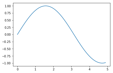
Plotting is straightforward. Again, let’s try Python first. Switch back to the Python kernel. Then try:

Note

In Jupyter notebooks, you typically need to use %matplotlib inline to display plots inline. In VS Code, this is handled automatically.

%matplotlib inline
import matplotlib.pyplot as p
import scipy as sc

x = sc.arange(0, 5, 0.1)
y = sc.sin(x)
p.plot(x, y)
p.xlabel('x')
p.ylabel('sin(x)')
p.title('A Simple Sine Wave')
p.show()

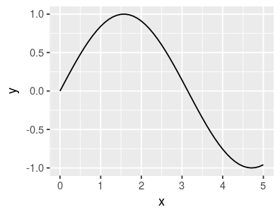
../_images/1f988677c6f93dddcace5d8142580df23e63e2896bca24dd015ce884650d7fc9.png

Now let’s try R. Switch to the R kernel, and try:

Tip

For interactive visualizations, you might also explore libraries like plotly (Python) or plotly for R, which create interactive plots that you can zoom, pan, and hover over.

require(ggplot2)
library(repr)# to resize plot within jupyter - this package is part of IRKernel
options(repr.plot.width=3.3,repr.plot.height=2.5)

x <- seq(0, 5, 0.1); y <- sin(x)
qplot(x, y, geom = "line") # large figure

Loading required package: ggplot2

../_images/7db6bb4aee94e64a0a21786665c51f3dbc3907761b9a01fc5142cb8501540098.png

Exiting a Jupyter Notebook#

Exiting is easy. Just CTRL+S (or Cmd+S on macOS) to save and close the browser. The server will still be active in the bash terminal. You may then relaunch by typing the local url (e.g., by typing http://localhost:8888/notebooks/MyJupyterNbName.ipynb) in your web browser window, or by exiting the kernel with CTRL+C (or Cmd+C on macOS) and then relaunching as you originally did.

Note

If you’re using VS Code, simply close the notebook tab. The kernel will stop automatically when VS Code closes, or you can manually stop it using the kernel status button in the top right of the notebook.

Congratulations!#

You’ve completed the introduction to Jupyter notebooks! You should now understand:

What Jupyter is and why it’s useful for scientific computing and literate programming
How to install and set up Jupyter on both Linux and macOS
Different ways to use Jupyter (classic notebook, JupyterLab, VS Code)
How to create, run, and manage notebooks
Best practices for creating reproducible, maintainable notebooks

Play around a bit with what you’ve learned. You can also try out the Data in Jupyter and Maths in Jupyter tutorials to continue learning.

Best Practices for Jupyter Notebooks#

As you develop your skills with Jupyter notebooks, following these best practices will help you create more maintainable, reproducible, and professional work:

Organization and Structure#

Use descriptive cell titles: Add markdown cells with headers to organize your notebook into logical sections
One concept per cell: Keep code cells focused on a single task or concept
Maintain logical flow: Execute cells in order from top to bottom; avoid jumping around
Document as you go: Add explanatory text before complex code blocks

Code Quality#

Import all libraries at the top: Keep all import statements in the first code cell
Use meaningful variable names: Avoid single letters except for common conventions (e.g., x, y for coordinates)
Add comments: Explain why you’re doing something, not just what you’re doing
Keep cells reasonably sized: If a cell is getting too long, consider breaking it up

Version Control#

Clear outputs before committing: Use “Clear All Outputs” before committing to git
- This keeps diffs clean and reduces file size
- In VS Code: Right-click notebook → “Clear All Outputs”
- In Jupyter: Kernel → Restart & Clear Output
Use .gitignore: Add common files to .gitignore:
```
.ipynb_checkpoints/
__pycache__/
*.pyc
```
Consider nbstripout: This tool automatically removes outputs when committing:
```
pip install nbstripout
nbstripout --install
```

Reproducibility#

Document your environment: Create a requirements.txt file:
```
pip freeze > requirements.txt
```
Set random seeds: When using random numbers, set seeds for reproducibility:
```
import numpy as np
np.random.seed(42)
```
Restart and run all: Periodically test that your notebook runs from start to finish:
- Kernel → Restart & Run All
Specify file paths carefully: Use relative paths and consider cross-platform compatibility:
```
from pathlib import Path
data_path = Path("../data/myfile.csv")
```

Performance and Resources#

Close notebooks when done: Notebooks continue to use memory even when idle
Monitor memory usage: Large datasets can exhaust memory; consider:
- Processing data in chunks
- Using data types efficiently (e.g., int32 instead of int64 when appropriate)
- Clearing large variables with del variable_name
Use %%time for profiling: Add %%time at the start of a cell to measure execution time

macOS-Specific Tips#

Use Cmd+S frequently: Save your work regularly (or enable auto-save)
Terminal integration: macOS terminal commands work in notebook cells with ! prefix:
```
!ls -la
!pwd
```
File paths: macOS uses forward slashes like Linux (/Users/...)
Hidden files: Use !ls -la to see hidden files starting with .

Tip

For coursework submissions, always run “Restart & Run All” before submitting to ensure your notebook executes correctly from top to bottom.

Introduction to Jupyter

Contents

Introduction to Jupyter#

What is Jupyter?#

Why use interactive notebooks?#

Key Jupyter features#

Jupyter vs. IPython#

Installing Jupyter#

Modern Jupyter Interfaces#

Installing and running jupyter in a virtual environment#

Ubuntu/Linux Installation#

macOS Installation#

Language Kernels#

Adding extensions to Jupyter#

Launching/Running a Jupyter Notebook#

Using tmux#

Detaching and Reattaching#

Why use tmux?#

Using Jupyter in VS Code#

Advantages of VS Code for Jupyter#

Setting Up Jupyter in VS Code#

Creating and Running Notebooks in VS Code#

VS Code-Specific Features#

Tips for macOS Users#

Key elements of the Jupyter nb content#

Text cells#

Equations#

Code cells#

Keyboard shortcuts#

Running code#

Graphics#

Exiting a Jupyter Notebook#

Congratulations!#

Best Practices for Jupyter Notebooks#

Organization and Structure#

Code Quality#

Version Control#

Reproducibility#

Performance and Resources#

Sharing and Collaboration#

macOS-Specific Tips#

Readings and Resources#

Using `tmux`#

Why use `tmux`?#