EnE Modelling and Advanced Data Science Pre-work#
Audience: Students taking the MQB Mathematical Modelling in E&E and Advanced Data Science sections
Tools (optional): NumPy, Matplotlib, SymPy.
Tip
How to use
Attempt the questions by hand first.
Use the optional Python cells to check algebra, plot functions, or verify numerical results.
Check your answers in the Solutions notebook.
1. Functions & graphs#
Focus: plotting, power laws, exponentials/logs, and trigonometric functions.
Exercise 1#
Radial disease spread (polynomial in time).
A fungal disease starts at the centre of an orchard and spreads radially at a constant speed \(v\) (m/day).
Write the infected radius \(r(t)\) and infected area \(A(t)\) as functions of time \(t\) (days).
Show that \(A(t)\) is a polynomial in \(t\), and state its degree.
If you measure time in weeks instead, \(t_w=t/7\), rewrite \(A\) as a function of \(t_w\).
Take \(v=3\) m/day and compute \(A(2)\), \(A(4)\), \(A(8)\) in m\(^2\).
Optional Python check:
import numpy as np

v = 3  # m/day
t = np.array([2,4,8], dtype=float)
r = v*t
A = np.pi*r**2
A
array([ 113.09733553, 452.38934212, 1809.55736847])
Exercise 2#
Allometric scaling (power laws).
Plant traits typically follow scaling relations [Niklas, 1994]. Suppose:
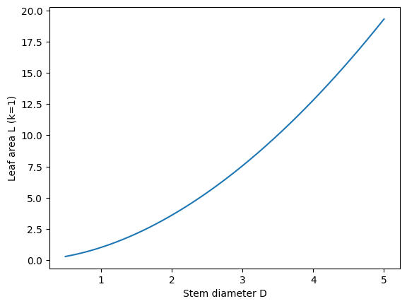
leaf area \(L\) is proportional to stem diameter \(D\) via \(L = k D^{1.84}\)
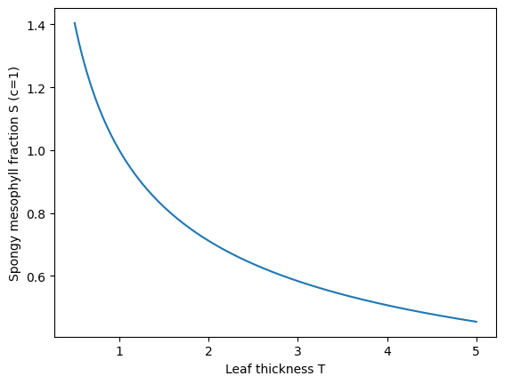
spongy mesophyll volume fraction \(S\) is proportional to leaf thickness \(T\) via \(S = c T^{-0.49}\)
Sketch (qualitatively) how \(L\) changes with \(D\), and how \(S\) changes with \(T\).
Using log–log axes, explain how you could estimate the exponent from data.
For \(k=1\), compute \(L\) when \(D=1,2,4\). For \(c=1\), compute \(S\) when \(T=1,2,4\).
Optional Python check:
import numpy as np
import matplotlib.pyplot as plt

D = np.linspace(0.5, 5, 200)
T = np.linspace(0.5, 5, 200)

L = D**1.84
S = T**(-0.49)

plt.figure()
plt.plot(D, L)
plt.xlabel("Stem diameter D")
plt.ylabel("Leaf area L (k=1)")
plt.show()

plt.figure()
plt.plot(T, S)
plt.xlabel("Leaf thickness T")
plt.ylabel("Spongy mesophyll fraction S (c=1)")
plt.show()
Exercise 3#
Exponentials, logs, and half-lives.
A bacterial population is exposed to a toxin; viable cells decline as \(N(t)=N_0(1/2)^{t/h}\), where \(h\) is the half-life.
Rewrite this as \(N(t)=N_0 e^{-\mu t}\) and express \(\mu\) in terms of \(h\).
If \(h=6\) hours and \(N_0=10^8\), compute \(N(3)\), \(N(6)\), \(N(12)\).
Explain (in words) what \(\mu\) represents biologically.
Optional Python check:
import numpy as np

N0 = 1e8
h = 6.0
t = np.array([3,6,12], dtype=float)

N = N0*(0.5)**(t/h)
N
array([70710678.11865476, 50000000. , 25000000. ])
Exercise 4#
Oscillations and seasonality.
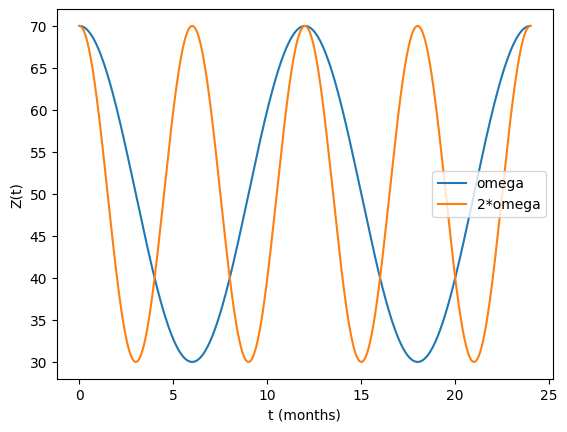
A zooplankton abundance time series shows seasonal oscillations. Model it as
Describe the role of \(Z_0\), \(A\), \(\omega\), and \(\phi\).
If the period is 12 months, what is \(\omega\) (in radians/month)?
Plot \(Z(t)\) over 24 months for \(Z_0=50\), \(A=20\), \(\phi=0\) and compare \(\omega\) vs \(2\omega\) (higher frequency).
Optional Python check:
import numpy as np
import matplotlib.pyplot as plt

Z0, A, phi = 50, 20, 0
t = np.linspace(0, 24, 1000)  # months
omega = 2*np.pi/12

Z1 = Z0 + A*np.cos(omega*t + phi)
Z2 = Z0 + A*np.cos(2*omega*t + phi)

plt.figure()
plt.plot(t, Z1, label="omega")
plt.plot(t, Z2, label="2*omega")
plt.xlabel("t (months)")
plt.ylabel("Z(t)")
plt.legend()
plt.show()
2. Calculus (limits, differentiation, integration, Taylor series)#
Focus: turning biological definitions into derivatives/integrals; approximations.
Exercise 1#
Limits and per-capita growth.
A population has size \(N(t)\). Define the instantaneous per-capita growth rate as
Show that \(r(t)=\frac{1}{N(t)}\frac{dN}{dt}\).
If \(N(t)=N_0 e^{rt}\), compute \(r(t)\) and interpret the result.
If \(N(t)\) is decreasing, what sign would you expect for \(r(t)\)?
Optional Python check:
import sympy as sp
t, r_sym, N0 = sp.symbols('t r N0', positive=True)
N = N0*sp.exp(r_sym*t)
r_of_t = sp.diff(N,t)/N
sp.simplify(r_of_t)
Exercise 2#
Differentiation and optimisation (resource uptake).
A microbial uptake rate follows a saturating function
where \(r\) is resource concentration.
Compute \(dU/dr\) and show it is positive.
Show that \(U(r)\to U_{\max}\) as \(r\to\infty\).
Find \(r\) such that \(U(r)=U_{\max}/2\) and interpret \(K\).
Optional Python check:
import sympy as sp
r, Umax, K = sp.symbols('r Umax K', positive=True)
U = Umax*r/(K+r)
dU = sp.diff(U, r)
sp.simplify(dU)
Exercise 3#
Integration (total biomass produced).
Suppose net primary production (NPP) in an ecosystem varies seasonally:
where \(t\) is time in years.
Compute the total production over one year: \(\int_0^1 \text{NPP}(t)\,dt\).
What is the average NPP over the year?
Explain why the cosine term integrates to zero over a whole number of periods.
Optional Python check:
import sympy as sp
t, a, b, omega = sp.symbols('t a b omega', positive=True)
NPP = a + b*sp.cos(omega*t)
sp.integrate(NPP, (t, 0, 1))
Exercise 4#
Taylor series (logistic growth approximation).
The logistic growth model is
For small \(N/K\), expand \(1-\frac{N}{K}\) and interpret the approximation.
Using a Taylor expansion of \(\ln(1+x)\) around \(x=0\), show how you would approximate \(\ln\left(1-\frac{N}{K}\right)\) when \(N\ll K\).
Explain (biologically) when this approximation might be justified.
Optional Python check:
import sympy as sp
x = sp.symbols('x')
sp.series(sp.log(1+x), x, 0, 4)
3. Linear algebra (matrices, eigenvalues/eigenvectors)#
Focus: matrix algebra for biological transitions/constraints; eigen-ideas for long-run behaviour.
Exercise 1#
Matrix multiplication in population transitions.
A 2-stage population (juveniles \(J\), adults \(A\)) evolves as
Interpret \(f, s, g\) biologically.
Compute \((J_{t+1},A_{t+1})\) for \(f=3\), \(s=0.2\), \(g=0.8\) given \((J_t,A_t)=(10,5)\).
Compute the matrix product explicitly (by hand), then verify with Python.
Optional Python check:
import numpy as np
M = np.array([[0, 3.0],[0.2, 0.8]])
x = np.array([10.0, 5.0])
M @ x
array([15., 6.])
Exercise 2#
Eigenvalues and long-run growth (Leslie-type model).
For the matrix \(M=\begin{pmatrix}0&3\\0.2&0.8\end{pmatrix}\):
Find the eigenvalues of \(M\).
Which eigenvalue determines the long-run growth rate, and why?
Find an eigenvector corresponding to the dominant eigenvalue and interpret it as a stable stage distribution (up to scaling).
Optional Python check:
import sympy as sp
M = sp.Matrix([[0, 3],[sp.Rational(1,5), sp.Rational(4,5)]])
M.eigenvects()
[(2/5 - sqrt(19)/5,
  1,
  [Matrix([
   [-sqrt(19) - 2],
   [            1]])]),
 (2/5 + sqrt(19)/5,
  1,
  [Matrix([
   [-2 + sqrt(19)],
   [            1]])])]
Exercise 3#
Inverses and solving linear systems (metabolic fluxes).
Suppose two metabolic fluxes \(x, y\) satisfy:
Write this as \(A\mathbf{z}=\mathbf{b}\).
Compute \(A^{-1}\) and hence \(\mathbf{z}=A^{-1}\mathbf{b}\).
Verify numerically.
Optional Python check:
import sympy as sp
A = sp.Matrix([[3,-7],[1,7]])
b = sp.Matrix([4,10])
z = A.LUsolve(b)
A.inv(), z
(Matrix([
 [  1/4,  1/4],
 [-1/28, 3/28]]),
 Matrix([
 [  7/2],
 [13/14]]))
Exercise 4#
Complex numbers and oscillations (optional stretch).
Many linear systems have solutions involving \(e^{(\alpha+i\beta)t}\).
Using Euler’s formula, show that \(e^{i\beta t}=\cos(\beta t)+i\sin(\beta t)\).
Explain why complex eigenvalues imply oscillations in real-valued solutions.
Consider \(x''+\beta^2 x=0\). Solve it using the Ansatz \(x(t)=e^{\lambda t}\) and relate \(\lambda\) to \(\pm i\beta\).
Optional Python check:
import sympy as sp
t, beta = sp.symbols('t beta', positive=True, real=True)
sp.exp(sp.I*beta*t).expand(complex=True)
4. Differential equations (equilibria, stability, phase-plane intuition)#
Focus: 1D and 2D dynamical systems used throughout quantitative biology.
Exercise 1#
Exponential growth ODE.
A bacterial population grows as \(\frac{dN}{dt}=rN\).
Solve for \(N(t)\) given \(N(0)=N_0\).
Define the doubling time \(T_d\) such that \(N(T_d)=2N_0\). Express \(T_d\) in terms of \(r\).
If \(r=0.4\ \text{h}^{-1}\), compute \(T_d\).
Optional Python check:
import sympy as sp
r = sp.Rational(2,5)  # 0.4
Td = sp.log(2)/r
float(Td)
1.7328679513998633
Exercise 2#
Logistic growth and equilibria.
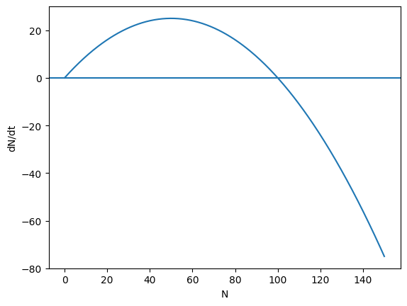
Find the equilibria.
Determine their stability by considering the sign of \(dN/dt\) around each equilibrium.
Sketch \(dN/dt\) as a function of \(N\).
Optional Python check:
import numpy as np
import matplotlib.pyplot as plt

r, K = 1.0, 100.0
N = np.linspace(0, 150, 400)
dN = r*N*(1 - N/K)

plt.figure()
plt.axhline(0)
plt.plot(N, dN)
plt.xlabel("N")
plt.ylabel("dN/dt")
plt.show()
Exercise 3#
Predator–prey linearisation (2D phase plane intuition).
A simplified predator–prey model near an equilibrium can be approximated by a linear system
Compute the eigenvalues of \(A\).
From the eigenvalues, classify the equilibrium (node/spiral/saddle) and predict whether trajectories oscillate.
(Optional) Simulate trajectories for a few initial conditions and plot \(y\) vs \(x\).
Optional Python check:
import numpy as np
import matplotlib.pyplot as plt

A = np.array([[0,1],[-2,-0.4]])
eigvals, eigvecs = np.linalg.eig(A)
eigvals
array([-0.2+1.4j, -0.2-1.4j])
Exercise 4#
Integrating factor (harvesting / forcing).
A fish stock \(N(t)\) experiences natural growth and constant harvesting:
with constants \(r>0\), \(H>0\).
Solve this ODE using an integrating factor.
Find the equilibrium \(N^*\) and interpret when it is biologically feasible.
If \(N(0)=N_0\), derive the condition on \(H\) for which the stock never crosses zero (no extinction in the deterministic model).
Optional Python check:
import sympy as sp
t, r, H, N0 = sp.symbols('t r H N0', positive=True)
N = sp.Function('N')
ode = sp.Eq(sp.diff(N(t), t), r*N(t) - H)
sp.dsolve(ode, ics={N(0): N0})
5. Probability & distributions#
Focus: expectation/variance and common distributions used in modelling and inference.
Exercise 1#
Random variables and expectation (offspring number).
Let \(X\) be the number of offspring produced by an individual in a season.
Define \(E[X]\) in terms of \(P(X=x)\).
If \(X\sim\text{Poisson}(\lambda)\), state \(E[X]\) and \(\mathrm{Var}(X)\).
If \(\lambda=1.5\), compute \(P(X=0)\), \(P(X\ge 2)\).
Optional Python check:
import numpy as np
import math

lam = 1.5
P0 = math.exp(-lam)
P1 = lam*math.exp(-lam)
Pge2 = 1 - (P0 + P1)
P0, Pge2
(0.22313016014842982, 0.44217459962892547)
Exercise 2#
Binomial sampling (infection prevalence).
In a sample of \(n\) hosts, each is infected with probability \(p\) independently. Let \(Y\sim\text{Binomial}(n,p)\).
State \(E[Y]\) and \(\mathrm{Var}(Y)\).
For \(n=50\), \(p=0.1\), compute \(E[Y]\), \(\mathrm{Var}(Y)\), and \(P(Y=0)\).
Interpret \(P(Y=0)\) in the context of field surveys.
Optional Python check:
import math
n, p = 50, 0.1
EY = n*p
VarY = n*p*(1-p)
P0 = (1-p)**n
EY, VarY, P0
(5.0, 4.5, 0.00515377520732012)
Exercise 3#
Gaussian measurement error (trait values).
Suppose measured leaf length \(L_m\) equals true length \(L\) plus error \(\epsilon\), where \(\epsilon\sim\mathcal{N}(0,\sigma^2)\).
Write the density of \(L_m\mid L\).
If you take \(k\) independent replicate measurements and average them, what happens to the variance of the average?
Explain why replication improves precision.
Optional Python check:
import sympy as sp
Lm, L, sigma = sp.symbols('Lm L sigma', positive=True, real=True)
pdf = (1/(sp.sqrt(2*sp.pi)*sigma))*sp.exp(-(Lm-L)**2/(2*sigma**2))
pdf
Exercise 4#
Joint, marginal, conditional probabilities (two species).
Two species (\(A\), \(B\)) can each be present (1) or absent (0) in a habitat patch.
Define a joint distribution \(P(A,B)\) over the four outcomes.
Show how to compute the marginal \(P(A=1)\) from \(P(A,B)\).
Define \(P(A=1\mid B=1)\).
Explain (in words) how \(P(A=1\mid B=1)\) relates to co-occurrence and (possible) interaction.
Optional Python check:
# Optional: pick numbers and verify marginals sum correctly
import numpy as np

# Example joint distribution table: rows A=0,1; cols B=0,1
P = np.array([[0.30, 0.10],
              [0.20, 0.40]])
P.sum(), P[1,:].sum(), P[:,1].sum(), P[1,1]/P[:,1].sum()
(np.float64(1.0),
 np.float64(0.6000000000000001),
 np.float64(0.5),
 np.float64(0.8))
6. Optimisation & likelihood#
Focus: interpreting likelihood spaces and optimisation over parameters (frequent pain points).
Exercise 1#
Minimising squared error (metabolic rate scaling).
You measure metabolic rate \(B\) and body mass \(M\) and hypothesise a power law \(B=aM^b\). Taking logs gives:
Let \(y_i=\log B_i\) and \(x_i=\log M_i\). Fit the line \(y=\beta_0+\beta_1 x\) by minimising
Take partial derivatives of \(S\) wrt \(\beta_0, \beta_1\) and write the normal equations.
Explain how this is an optimisation problem over a 2D parameter space.
(Optional) Solve the normal equations for \((\beta_0,\beta_1)\) in terms of sample means.
Optional Python check:
import sympy as sp
b0, b1 = sp.symbols('b0 b1')
# symbolic normal equations for generic data would be done by writing sums; see solutions notebook for steps.
Exercise 2#
Likelihood surface (single-parameter Poisson).
You observe counts of offspring per individual: \(x_1,\dots,x_n\), and model them as Poisson(\(\lambda\)).
Write the likelihood \(L(\lambda)\) and log-likelihood \(\ell(\lambda)\).
Differentiate \(\ell(\lambda)\) and find the MLE \(\hat\lambda\).
Explain what the “height” of a 1D likelihood curve represents.
For data \([0,1,0,2,1]\), compute \(\hat\lambda\) and plot \(\ell(\lambda)\) for \(\lambda\in[0.01,4]\).
Optional Python check:
import numpy as np
import matplotlib.pyplot as plt

x = np.array([0,1,0,2,1])
lam_hat = x.mean()

lam = np.linspace(0.01, 4, 500)
# log-likelihood up to an additive constant (drop -log(x_i!))
ell = (x.sum())*np.log(lam) - len(x)*lam

plt.figure()
plt.plot(lam, ell)
plt.axvline(lam_hat, linestyle='--')
plt.xlabel("lambda")
plt.ylabel("log-likelihood (up to constant)")
plt.show()

lam_hat
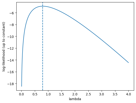
np.float64(0.8)
Exercise 3#
Two-parameter likelihood and contours (Gaussian mean/variance).
Suppose trait measurements \(y_1,\dots,y_n\) are i.i.d. Normal(\(\mu,\sigma^2\)).
Write the log-likelihood \(\ell(\mu,\sigma)\).
State the MLEs \(\hat\mu\) and \(\hat\sigma^2\).
Explain why a 2D likelihood can be visualised via contour lines over \((\mu,\sigma)\).
(Optional) For data \([2.1, 2.4, 1.9, 2.0, 2.3]\), plot a contour map of \(\ell(\mu,\sigma)\).
Optional Python check:
import numpy as np
import matplotlib.pyplot as plt

y = np.array([2.1, 2.4, 1.9, 2.0, 2.3])
mu_grid = np.linspace(1.8, 2.6, 120)
sig_grid = np.linspace(0.05, 0.6, 120)
MU, SIG = np.meshgrid(mu_grid, sig_grid)

n = len(y)
# log-likelihood
LL = -n*np.log(SIG) - 0.5*np.sum(((y.reshape(1,1,-1)-MU[...,None])/SIG[...,None])**2, axis=-1)

plt.figure()
cs = plt.contour(MU, SIG, LL, levels=15)
plt.clabel(cs, inline=True, fontsize=8)
plt.xlabel("mu")
plt.ylabel("sigma")
plt.show()

y.mean(), y.std(ddof=0)
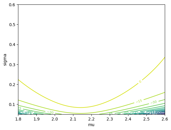
(np.float64(2.1399999999999997), np.float64(0.18547236990991403))
Exercise 4#
Constraints (biologically feasible parameter values).
In many models parameters must be positive (rates, variances, concentrations).
Give two examples of biological parameters that are constrained to be \(>0\).
Suppose you are fitting \(N(t)=N_0e^{- \mu t}\) but your optimiser returns \(\mu<0\). What biological behaviour would that imply?
Show how to reparameterise \(\mu=e^\theta\) to enforce positivity, and explain how this changes the optimisation problem.
Optional Python check:
import sympy as sp
theta = sp.symbols('theta', real=True)
mu = sp.exp(theta)
mu